TDM-深度树匹配

发表于 2019-08-12 | 分类于 Tool ， match |

之前介绍过基于乘积量化方式PQ构建分库索引的fasis工具解决召回效率低的问题，本文介绍一种基于树的高效匹配算法。我们在数据结构上知道搜索二叉树BST等系列的树查找时间复杂度是对数级别，knn based的一些检索结构KD树等都是检索比较高效的数据结构，通过分而治之的方式进行不断查找。基于树这样的天生的优良特性，阿里妈妈的作者们在推荐领域下，提出TDM算法解决全库检索效率低和推荐系统两阶段分割的问题。针对召回和排序两阶段联合为一个阶段是目前的一个大趋势，而本文重点关注的是如何高效地进行全库检索。下文为个人解读的主要梳理部分

问题背景：某某场景下，加速全库匹配过程

文章：

TDM一期：Learning Tree-based Deep Model for Recommender Systems

TDM二期：Joint Optimization of Tree-based Index and Deep Model for Recommender Systems

代码：https://github.com/alibaba/x-deeplearning/tree/master/xdl-algorithm-solution/TDM

离线训练： https://github.com/alibaba/x-deeplearning/wiki/深度树匹配模型(TDM)
在线Serving：https://github.com/alibaba/x-deeplearning/wiki/TDMServing

来源：参考人脑，兴趣的建立由粗到细的组织方式和检索方法，比如10亿的商品列表，只需要30次的查找

How: 为什么检索出来的top-k，就是用户感兴趣的 Topk?有效性如何去保证？有效性检索的建模背后隐藏着对用户兴趣的建模。

基础结构：用户兴趣的最大堆树，首先是定义第j层用户对节点n的兴趣为用户对对节点n的子节点层下j+1的兴趣最大值。

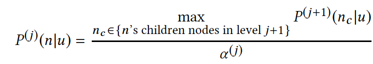
由于是递归定义，具有性质：最大堆树下，当前层最优 TopK 节点的父亲，一定属于上一层的最优 TopK。

扩展点：这里的max操作可以如何去替换？min, all??

举例如下：

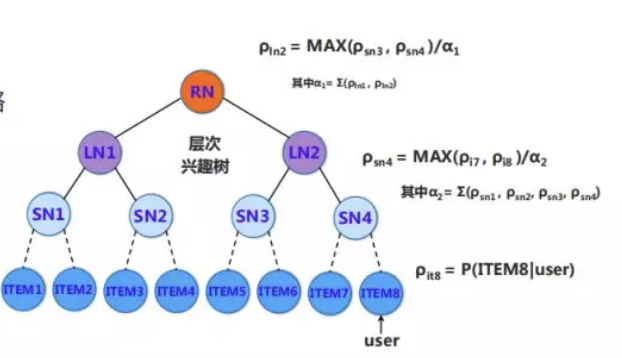
如果item6和item8是全局的最优top2节点，那么SN层中SN3和SN4是最优的top2.

由此可见，用户兴趣的最大堆树的定义是保证这种检索(beam seach)有效的充分条件，所以实际做的过程可以从根节点出发，逐层选择top-k,一直到叶子节点。

既然最大堆树的定义保证这种检索的有效性，那么这棵树应该如何去学习？

从检索本质看，针对具体的某一层，beam search检索过程需要保证当前层检索层具有top k排序的能力。

整体的思路：构建符合这样性质的样本，让样本牵引模型学习，去逼近最大堆。

具体的做法：主要分叶子层的节点兴趣和中间层的节点兴趣两部分进行构建。叶子层的节点兴趣，从用户的直接行为产生，对应着感兴趣和不感兴趣。中间层的兴趣节点，用最大堆递归上述的方式去推导每一层的序标签，当我们有了每一层的序标签，就可以用深度学习去拟合序标签的样本。

TensorFlow中使用CRF

发表于 2019-08-02 | 分类于 Tool ， CRF |

背景：关于CRF的应用，尤其是在深度学习之前它是一个nlp序列建模的比较主流方法，即使是深度学习大行其道，也会出现crf的影子，比如bilstm+crf, bert+crf. 关于crf的原理可参考众多的资料，本文提供一个在tensorflow中使用crf的一个简要概述。

CRF使用的主要API

crf_log_likelihood

def crf_log_likelihood(inputs,
                       tag_indices,
                       sequence_lengths,
                       transition_params=None):
  """Computes the log-likelihood of tag sequences in a CRF.
  Args:
    inputs: A [batch_size, max_seq_len, num_tags] tensor of unary potentials
        to use as input to the CRF layer.
    tag_indices: A [batch_size, max_seq_len] matrix of tag indices for which we
        compute the log-likelihood.
    sequence_lengths: A [batch_size] vector of true sequence lengths.
    transition_params: A [num_tags, num_tags] transition matrix, if available.
  Returns:
    log_likelihood: A [batch_size] `Tensor` containing the log-likelihood of
      each example, given the sequence of tag indices.
    transition_params: A [num_tags, num_tags] transition matrix. This is either
        provided by the caller or created in this function.
  """

输入：

inputs，一元势能得分，针对每个word级别，每个标签的预测概率值，<句子长度,标签大小>的tensor
tag_indices：真实标签的序列，<句子长度,标签大小>的tensor
sequence_lengths：实际标签序列的长度，为一个值
transition_params：标签状态转移矩阵，学习的参数矩阵，可以预先给定

输出：

log_likelihood，word级别的对数似然概率
transition_params：学习后的状态转移矩阵

解码过程的两个可用的API
- tf.contrib.crf.viterbi_decode(tf_unaryscores, tf_transition_params)
- tf.contrib.crf.crf_decode(unary_scores, transition_params, sequence_lengths)

一个具体的例子：

import numpy as np
import tensorflow as tf
# Data settings.
num_examples = 10
num_words = 20
num_features = 100
num_tags = 5
# Random features.
x = np.random.rand(num_examples, num_words, num_features).astype(np.float32)
# Random tag indices representing the gold sequence.
y = np.random.randint(num_tags, size=[num_examples, num_words]).astype(np.int32)
# All sequences in this example have the same length, but they can be variable in a real model.
sequence_lengths = np.full(num_examples, num_words - 1, dtype=np.int32)
# Train and evaluate the model.
with tf.Graph().as_default():
  with tf.Session() as session:
    # Add the data to the TensorFlow graph.
    x_t = tf.constant(x)
    y_t = tf.constant(y)
    sequence_lengths_t = tf.constant(sequence_lengths)
    # Compute unary scores from a linear layer.
    weights = tf.get_variable("weights", [num_features, num_tags])
    matricized_x_t = tf.reshape(x_t, [-1, num_features])
    matricized_unary_scores = tf.matmul(matricized_x_t, weights)
    unary_scores = tf.reshape(matricized_unary_scores,
                              [num_examples, num_words, num_tags])
    # Compute the log-likelihood of the gold sequences and keep the transition
    # params for inference at test time.
    log_likelihood, transition_params = tf.contrib.crf.crf_log_likelihood(
        unary_scores, y_t, sequence_lengths_t)
    # Compute the viterbi sequence and score.
    viterbi_sequence, viterbi_score = tf.contrib.crf.crf_decode(
        unary_scores, transition_params, sequence_lengths_t)
    # Add a training op to tune the parameters.
    loss = tf.reduce_mean(-log_likelihood)
    train_op = tf.train.GradientDescentOptimizer(0.01).minimize(loss)
    session.run(tf.global_variables_initializer())
    mask = (np.expand_dims(np.arange(num_words), axis=0) <
            np.expand_dims(sequence_lengths, axis=1))
    total_labels = np.sum(sequence_lengths)
    # Train for a fixed number of iterations.
    for i in range(1000):
      tf_viterbi_sequence, _ = session.run([viterbi_sequence, train_op])
      if i % 100 == 0:
        correct_labels = np.sum((y == tf_viterbi_sequence) * mask)
        accuracy = 100.0 * correct_labels / float(total_labels)
        print("Accuracy: %.2f%%" % accuracy)

CRF 编码/训练逻辑

获得表示：获得原始的model产出，比如lstm或者bert的表示，<句子长度,隐藏大小>的tensor.
计算每个word得分/全局的一元势函数(global unary potential)：加入Project映射层计算每个word的得分，输出的大小为<句子长度,标签大小>
Train: 使用crf_log_likelihood进行极大似然估计的train,这里可以标签的转移矩阵需要学习，是一个参数矩阵，得到一个log_likelihood和标签状态转移表示(decode用)

log_likelihood, transition_params = tf.contrib.crf.crf_log_likelihood(
unary_scores, gold_tags, sequence_lengths, trans)
在word级别上累加计算loss

loss = tf.reduce_mean(-log_likelihood)

选择具体的优化算法进行学习

1	train_op = tf.train.GradientDescentOptimizer(0.01).minimize(loss)

CRF 解码/测试逻辑

一种可以使用crf_decode的tf代码进行解码，另外一种使用Numpy代码的viterbi_decode解码方式

numpy的解码风格:

tf_unary_scores, tf_sequence_lengths, tf_transition_params, _ = session.run([unary_scores, sequence_lengths, transition_params, train_op])
for tf_unary_scores_, tf_sequence_length_ in zip(tf_unary_scores, tf_sequence_lengths):
    # Remove padding.
    tf_unary_scores_ = tf_unary_scores_[:tf_sequence_length_]
    # Compute the highest score and its tag sequence.
    tf_viterbi_sequence, tf_viterbi_score = tf.contrib.crf.viterbi_decode(
        tf_unary_scores_, tf_transition_params)

TF的风格

1
2
3

viterbi_sequence, viterbi_score = tf.contrib.crf.crf_decode(unary_scores, transition_params, sequence_lengths)
tf_viterbi_sequence, tf_viterbi_score, _ = session.run([viterbi_sequence, viterbi_score, train_op])

主要逻辑：

通过crf正向过程获得标签状态转移的参数transition_params。

log_likelihood, transition_params = tf.contrib.crf.crf_log_likelihood(
unary_scores, gold_tags, sequence_lengths)
尝试上面介绍的任意一种解码的风格，输入参数都是transition_params和unary_scores一元势能函数，得到具体的解码序列

要点：

1.transition_params标都是来自于crf_log_likelihood的第二个输出值

1 2	log_likelihood, transition_params = tf.contrib.crf.crf_log_likelihood( unary_scores, gold_tags, sequence_lengths)

2.unary_scores，是针对每个词的输入的得分(一元势能函数得分)，维度大小是<句子长度, 标签大小>，一般来源都是经过了一个project层/全联接层，比如

bi-lstm, 输出为 <句子长度,2倍隐藏大小>, 这时需要一个映射层<2倍隐藏大小,标签大小>，转化为针对每个word的<句子长度, 标签大小>.
Bert,输出为<句子长度，隐层大小768>, 这时需要一个映射层<隐层大小,标签大小>，转化为针对每个word的<句子长度, 标签大小>.

3.训练过程和测试/解码过程都需要传入句子的实际长度的参数，主要是针对输入的长度进行了padding为最长，测试统计的时候要去掉这个部分。

相似性搜索工具-Faiss

发表于 2019-07-30 | 分类于 Tool ， match |

Faiss

背景

目标：在千万规模的数据上，高效计算内积/相似性，返回top-K个结果

文章：Billion-scale similarity search with GPUs

代码：https://github.com/facebookresearch/faiss

简介：

时间、质量和训练速度的权衡。
Faiss 是一个用于有效的相似性搜索和密集向量聚类的库。其包含了在任何大小（甚至可以大到装不进 RAM）的向量集中进行搜索的算法。其也包含用于评估和参数调整的支持性代码。
Faiss 是围绕一种存储了一个向量集的索引类型（index type）而构建的，并且提供了一个使用 L2 或点积向量比较在其中进行搜索的函数。

方法：提出了一种用于 k-selection 的设计，其可以以高达理论峰值性能 55% 的速度进行运算，从而实现了比之前最佳的 GPU 方法快 8.5 倍的最近邻KNN搜索。另外，基于积量化（product quantization）的暴力计算、近似和压缩域搜索（compressed-domain search）提出优化过的设计，从而将其应用到了不同的相似性搜索场景中。

效果： 35 分钟内从 Yfcc100M 数据集的 9500 万张图像上构建一个高准确度的 k-NN 图（graph），也可以在 12 个小时内在 4 个 Maxwell Titan X GPU 上构建一个连接了 10 亿个向量的图。

实现细节：

WarpSelect：文中提出的 k-selection 的设计，完全在寄存器（register）中维持状态，且仅需要在数据上进行单次通过，从而避免了 cross-warp synchronization，使用merge-odd 和 sort-odd 作为原语。

WarpSelect的整体流程如下：
针对特定lane j的流程如下：

使用方法

安装：pip install faiss-cpu
使用示例：https://github.com/facebookresearch/faiss/wiki/Getting-started
- 准备数据
- 构建索引：可以选择的索引格式为https://github.com/facebookresearch/faiss/wiki/Faiss-indexes
- 搜索查询：search(query, top-k)
加速搜索的一些技巧：https://github.com/facebookresearch/faiss/wiki/Faster-search
- 使用复合的索引：https://github.com/facebookresearch/faiss/wiki/Faiss-indexes-(composite)
- IndexFlatL2 和 IndexIVFFlat都要存储所有的向量数据，对于大型数据集是不现实的, Faiss基于PQ提供了变体IndexIVFPQ来压缩数据向量（一定的精度损耗）

参考资料

Faiss教程：入门
Faiss的基础使用：https://waltyou.github.io/Faiss-Introduce/
Faiss Indexs 的进一步了解：https://waltyou.github.io/Faiss-Indexs/
向量检索在闲鱼视频去重的实践：https://zhuanlan.zhihu.com/p/43972326
阿里BE引擎深度集成开源的KNN库–FAISS
改造定制使其支持向量索引的分布式构建和查询，实现多种基于量化的方法如粗量化、积量化以及粗量化 + 积量化的组合等方法，并且在线查询的延时、索引构建的性能都很优秀。

机器学习基础夯实系列-贝叶斯优化

发表于 2019-07-21 | 分类于机器学习基础 |

贝叶斯优化小结

背景

针对通用的函数求最小化的问题 $x∗=argmin{x∈X}f(x)$ ，如果定义域X是凸集和函数f是凸函数，可以采用凸优化的思路得到最优值,而针对非凸函数，f的一次运算需要大量的资源。通常此时可以采用贝叶斯优化的思路

基本思想

首先对f(x)有一个猜想的先验分布模型PF，然后利用后续新获取到的信息，来不断优化那个猜想模型，使模型越来越接近真实的分布

主要方法

SMBO

Sequential model-based optimization (SMBO) 是贝叶斯优化的最简形式

主要过程

1.输入步：Input: f黑盒子函数，X训练数据，S为Acquisition Function，M为是基于输入数据假设的模型，即已知的输入数据x都是在这个模型上的，可以用来假设的模型有很多种，例如随机森林，Tree Parzen Estimators，常见的比如GP高斯分布过程。

2.初始化步(构建示例)：初始化获取数据InitSamples(f,X), $D={(x_i,yi)}{i=1}^{n}$,其中每一个$y_i$为已知的, 即$y_i=f(x_i)$

3.迭代步：
3.1 $p(y|x,D) <- FitModel(M, D)$ 使用猜想的分布模型M(比如高斯分布) 在特定的数据下进行训练。由于输入服从高斯分布，那么可以知道其预测也是服从高斯分布的。这里实质计算计算高斯分布的主要参数估计的均值和方差。

3.2.基于估计的假定模型M(高斯分布)去选择当前轮的输入$x_i$,基本思想就是选择收益最高的点。主要是利用Acquisition Function函数。acquisition function是一个权衡exploritation和exploration的函数。

1) Optimistic policies , 主要采用上限置信区间（upper confidence bound）。常用的如GP-UCB等方法

2) Information-based policies,主要思想是利用后验信息来进行选点。常用有Thompson sampling 和 entropy search。基于熵的方法感觉发展空间还比较大，有一些相关工作都有用到这个。

3) Portfolios of acquisition functions

这类方法就是将多种AC方法进行集成，最近的工作比如有ESP

4）Expected improvement(EI)

可以在explore和explot之间平衡，explore时选择均值大的点,exploit选择方差大的点

5） Probability of improvement(POI)

新的采样能提升最大值的概率最大， MPI（maximum probability of improvement)，或P算法

3.3 使用新样本进行模型训练，此步骤比较耗时

3.4 训练实例的更新

应用

LDA、组合优化、自动机器学习、增强学习、气象、机器人等等

参考资料

1.https://blog.csdn.net/Snail_Ren/article/details/79005069

2.https://github.com/tobegit3hub/advisor Google内部的Vizier调参服务以及其开源实现Advisor项目

3.https://zhuanlan.zhihu.com/p/29779000 贝叶斯优化: 一种更好的超参数调优方式

4.贝叶斯参数调优实战：https://www.jianshu.com/p/4c0cef6176fa

知识蒸馏-Knowledge Distillation

发表于 2019-07-11 | 分类于模型压缩， Distillation |

基础介绍

核心思想

KD（Distilling the Knowledge），就是用teacher network的输出作为soft label(target)来训练一个student network。

Knowledge Distill是一种简单弥补分类问题监督信号不足的办法. 常见的监督信号表示hard target,是0-1的表示，而KD的表示从soft target学习，拥有不同类之间关系的信息（比如同时分类驴和马的时候，尽管某张图片是马，但是soft target就不会像hard target 那样只有马的index处的值为1，其余为0，而是在驴的部分也会有概率。）
知识蒸馏是一种模型压缩常见方法，用于模型压缩指的是在teacher-student框架中，将复杂、学习能力强的网络学到的特征表示“知识”蒸馏出来，传递给参数量小、学习能力弱的网络。

Loss表达

Loss的表达：$L=\alpha L{soft}+(1−\alpha)L{hard}$
distillation loss选择：平方距离，KL-divergence，cross entropy。

核心结构：

实现问题思考

1.student网络的具体形态的选择？很多方式，可以异质也可以同质的

2.teacher网络的结构，选择几个分类器，因为数据集上不同个数的分类器性能不一样

3.teacher预测错误的知识需要单独剔除吗？

4.当类别少的时候效果就不太显著，对于非分类问题也不适用？

常见的T-S形态

Case1:

teacher：WRN-40-10

student: WRN-10-4(CIFAR)/WRN-22-4(Imagenet32)

Case2:

Teacher:BERT-Base

Student:3层BERT / BiLSTMAttn+TextCNN

参考资料

简评 | 知识蒸馏（Knowledge Distillation）最新进展（一）
简评 | 知识蒸馏（Knowledge Distillation）最新进展（二）
如何理解soft target这一做法？
soft target的作用在于generalization。同dropout、L2 regularization、pre-train有相同作用。
知识蒸馏（Knowledge Distillation

音频特征抽取

发表于 2019-07-09 | 分类于 Tool ， Audio |

背景

原材料：视频文件(signed 16-bit PCM)/音频

工具：VGGish/ffmpeg

任务：抽取音频文件的embedding语义向量.

下载地址：https://github.com/tensorflow/models/tree/master/research/audioset/vggish

VGGish基础介绍

在AudioSet是Google发行的声音版ImageNet上训练得到预训练模型，该模型可以将音频文件抽取为128维度的语义向量，除了直接抽取特征外，还可以进行针对特定的任务进行FineTuning操作。

VGGish vs VGG

VGGish是 VGG的变体，含有11个权重层，具体有如下改变：

输入大小修改为96x64，log mel spectrogram的音频输入
去掉了最后一组的conv和pool层，有4组结构而不是5组e.
全联接层(compact embedding层)不是想image那样使用1000而是使用的是128维度的.

VGGish依赖包

VGGish文件结构：

vggish_slim.py: Model definition in TensorFlow Slim notation.
vggish_params.py: Hyperparameters.
vggish_input.py: Converter from audio waveform into input examples.
mel_features.py: Audio feature extraction helpers.
vggish_postprocess.py: Embedding postprocessing.
vggish_inference_demo.py: Demo of VGGish in inference mode.
vggish_train_demo.py: Demo of VGGish in training mode.
vggish_smoke_test.py: Simple test of a VGGish installation

VGGish使用介绍

音频文件：signed 16-bit PCM samples

使用示例: vggish_inference_demo.py

计算log mel spectrogram()
examples_batch = vggish_input.wavfile_to_examples(wav_file)
vggish抽取

features_tensor = sess.graph.get_tensor_by_name(vggish_params.INPUT_TENSOR_NAME)
embedding_tensor = sess.graph.get_tensor_by_name(vggish_params.OUTPUT_TENSOR_NAME)[embedding_batch] = sess.run([embedding_tensor], feed_dict={features_tensor: examples_batch})
后处理

PCA变换+8bit定点化

VGGish was trained with audio features computed as follows:

All audio is resampled to 16 kHz mono.
A spectrogram is computed using magnitudes of the Short-Time Fourier Transform with a window size of 25 ms, a window hop of 10 ms, and a periodic Hann window.
A mel spectrogram is computed by mapping the spectrogram to 64 mel bins covering the range 125-7500 Hz.
A stabilized log mel spectrogram is computed by applying log(mel-spectrum + 0.01) where the offset is used to avoid taking a logarithm of zero.
These features are then framed into non-overlapping examples of 0.96 seconds, where each example covers 64 mel bands and 96 frames of 10 ms each.

视频抽取音频

ffmpeg -y -i xxx.mp4 -ar 16000 -ac 1 xxx.wav

主要参数含义：

-y: 覆盖输出的文件

-ar rate set audio sampling rate (in Hz)
-ac channels set number of audio channels

参考

Gemmeke, J. et. al., AudioSet: An ontology and human-labelled dataset for audio events, ICASSP 2017
Hershey, S. et. al., CNN Architectures for Large-Scale Audio Classification, ICASSP 2017
https://github.com/tensorflow/models/tree/master/research/audioset

虚拟对抗训练

发表于 2019-07-08 | 分类于 GAN ，虚拟对抗训练 |

虚拟对抗训练(VAT): 全称为Virtual Adversarial Training,核心思想是在监督学习中对抗部分，采取的措施可以是加噪音增强鲁棒性、对抗具体的分布等，联合对抗部分loss一起训练。

1.Word Embedding Perturbation for Sentence Classification

在答案选择、关系分类、情感分类上，在word embedding上面实现对抗

code:https://github.com/zhangdongxu/word-embedding-perturbation

2.Adversarial Personalized Ranking for Recommendation

VAT是在对抗训练的基础上将监督学习模型扩展到半监督学习模型，同时模型在同向噪声鲁棒性提高到可以在异向噪声具有鲁棒性，在监督和半监督条件下都取得不错的实验结果。

3. Virtual Adversarial Training: a Regularization Method for Supervised and Semi-supervised Learning

利用对抗的思想，要求模型对一个样本在施加对抗性噪声前后给出尽可能相同的预测值，从而对模型施加 smooth regularization，以此利用无标注样本进行半监督学习。论文仅用 100 个标注 MNIST 样本取得 1.36% 的测试误差，仅用 4000 个标注 CIFAR 样本取得 13.15% 的测试误差。

Code

4.Adversarial Dropout for Supervised and Semi-supervised Learning

Virtual Adverarial Training的变种，原来在 input data 上加对抗干扰，本文在网络中间层进行对抗性 dropout，取得了与 VAT 接近的半监督训练效果，配合原始 VAT 一起在 CIFAR 和 SVHN 上取得 state-of-the-art 的半监督学习性能

5.Distributional Smoothing with Virtual Adversarial Training

局部分布性平滑(LDS) 的方法，这是统计模型的一个新的光滑概念，可以用作正则化术语来促进模型分布的平滑

CRF使用的主要API

CRF 编码/训练逻辑

CRF 解码/测试逻辑

Faiss

背景

使用方法

参考资料

贝叶斯优化小结

背景

基本思想

主要方法

SMBO

主要过程

应用

参考资料

基础介绍

核心思想

Loss表达

核心结构：

相关文章调研

实现问题思考

参考资料

背景

VGGish基础介绍

VGGish vs VGG

VGGish依赖包

VGGish文件结构：

VGGish使用介绍

视频抽取音频

参考

BERT在推荐系统的梳理

GAN在推荐中应用梳理

IRGAN

GraphGAN

CFGAN

RAGAN

APR

Adversarial Recommendation: Attack of the Learned Fake Users

主要文章

重点解读

Generative Adversarial User Model for Reinforcement Learning Based Recommendation System，蚂蚁金服，ICML 2019